RGrace package for R Statistical System.
Note Please!
This package is a replacement for older package Disgrace. RGrace works under R-1.9.1 and grid
package shipped with it. If you use older version of R then you have 2
options - either upgrade or use Disgrace
(although the support for this one is discontinued).
Purpose.
RGrace is a package for creation of simple every-day
diagramms and charts, although it is suited for production of
publiction-quality scientific graphics. It combines easy to use
point-and-click interface, ability to interact with graphic with mouse
clicks and drags and possibility to incorporate rather sophisticated
R-scripts in the process of plotting. It is written (almost) entirly in
R language (as it heavily depends on environment() I think it is not
compatible with S-language) and use GTK (ver. 1.2.x ) as a front end
toolkit.
It is named after Grace
charting application which I tried to emulate.
Screenshots.
If you like screenshots I have some:
Simple chart with R-session in Emacs
Text annotations, multiple panels and
postscript output.
Various data line styles and saved
figure's file.
The same figure zoomed.
Fancy axis ticks labels in Russian.
Composite multilined text annotation AKA
legend (ver. 0.2.4)
Pdf-file with outlined cyrillic fonts
made from RPlots.ps with ps2pdf (ver. 0.2.5)
Main window with an Industrial theme and
GTK2.0 toolkit (ver. 0.3-4)
Copying panels from example(ggplot)
between different figures (ver. 0.4-3)
RGrace output over x11 graphic
device(ver. 0.4-6)
Database interface (ver. 0.5-0)
Installation
To install RGrace package you need GTK-1.2 system library (www.gtk.org) already installed on your
computer. Of course you will need R
Statistical System and I highly recommend to install an Emacs
Speaks Statistics package - it makes a process of developing R
scripts under Emacs a lot easier.
And last but not least - you will need Linux. This package is tested
and supported under Linux only (!).
If you wants to be on the bleeding edge of R and RGrace development
install the R-devel source and compile it. To download r-devel source
tree the best way is to use rsync (be sure that your firewall does not
block 873 port):
mkdir R-devel
rsync -rC --delete
rsync.R-project.org::r-devel R-devel
Then - cd R-devel ; ./configure ;
make ; make install
After that download http://www.omegahat.org/RGtk/RGtk_0.6-15.tar.gz
, and get from nearest mirror of CRAN new gtkDevice package (version
1.9-2 and higher, older versions wouldn't work!). As an option you can
use development version of gtkDevice
(0.5-4 with changes made by Paul Murrel), it seems to me the newer
version behaves strangely when switching between graphic devices.
Install them under root account in this sequence (only after R was
succesfully installed!):
R INSTALL -c RGtk_0.6-14.tar.gz
R INSTALL gtkDevice_1.9-2.tar.gz
After this is done you can
install RGrace package -
R INSTALL RGrace_0.4-<x>.tar.gz
(substitute x with actual RGrace version!)
If R INSTALL RGrace_... fails first check Makevars file in src
sub-directory. In this file paths to gtk, glib and gdk includes and
libraries are specified. Edit them to match your system installation.
After that you are ready to enjoy RGrace and to send bug-reports to me
;)
There used to be a port of RGrace to Gtk2 (with home-made Gtk2 binding
to R-language - adaptation of Duncan Temple Lang RGtk package). But it
proves to be a nightmare the way locales are handled in Gtk2 (which is
fully utf8 now) and R, so I lay it off for some time until I will be
ready to drop KOI8-R locale, I am used to, in favour of UTF8 one. If you
are interested, results of my experiments as well as some tips on
installing and running it you can find here.
Downloads
RGrace_0.5_4
Stable release
Changelog
Kick-start.
Run R and issue command library(RGrace).
After that you can call plotting window by command figure() or plot
something at once by command ggplot(c(1,2,3,4),c(1,2,3,4)) (or any other
numerical vectors). ggplot() is a shortcut for figure()$panel(
)$element(c(1,2,3,4),c(1,2,3,4)).
When data is plotted you may change its appearence by GUI controls that
are located at slide panel to the left of plotting area.
GUI Help.
Note Please! This information is quite
outdated and will soon be removed from this site. For valid information
look into RGrace manpages, i.e. library(help=RGrace).
Some "theory". You can have in R sessiom multiple figure()'s, in each of them may be
severals panel()'s and in each
panel (i.e. 4 axes with labels and tags) may be several data curves
("elements") and text annotations bound to these axes coordinate system
("native units" in terms of grid package). In every moment only one of
figures is active and current.Figure
global variable holds currently active figure. "Current panel" may be
chosen by combo box in this figure or selected from console by
command current.Figure$panel(select=x)
where x is panel number and x corresponds to position of this panel in
combobox. Plotting is done by command ggplot(x,y)
with suitable data vectors x,y and output of this command will be
directed to current panel inside current.Figure(if
either of them does not exist it will be created). You can in any time
create blank figure or panel by command figure()->fig and fig$panel() and assign returned
values to variables (this functions has an side effect of setting current.Figure and "current panel"
to returned values). Say you have created panel as current.Figure$panel()->SavedPanel. Then
in any time you may add plot to SavedPanel
(irrespective what "current panel" is) by command SavedPanel$element(x,y) (should I
mention what SavedPanel$element(select=num)
return you a element's "handle" for editing/contemplating?).
Selecting/setting annotations works just the same - SavedPanel$annotation("test label",x=1,y=1)
(or SavedPanel$annotation(label=list("test
label",expression(frac(x,y))),x=1,y=1) - for multilined text)
to add annotation and SavedPanel$annotation(select=num)
to select an existing num'th one. Figure selecting can not be done
through command line (DO NOT do asignments to current.Figure variable !) but
usually this is not needed - then you edit plots, panels, annotations
through GUI current.Figure is
set to the figure you will expect changes will be applyed to.
The most obvious side effect of all these commands is
graphic output produced in drawing area of the figure and also changes
in GUI controls located on left hand slide panel (then you first opens
figure slide panel is collapsed and you should drag its handle to make
it visible).
It has a notebook with "Panels", "Elements", "Annotations" pages and
short menu. Let us look at the notebook:
Panels.
Here you can select and edit properties of panels(axes) located in this
figure.
"Apply" button - changes you
made in GUI controls are submitted to panel after this button is pressed.
"Add New" button - add new blank
panel with default values. Make it the current one.
"Delete" button - delete the
current panel.
"Autorange" button - rescales
current panel so all elements in it will be shown.
Unnamed combo box - list of
panels in this figure. Selecting entry in it made selected panel
current. Also updates GUI controls with the panel properties values.
"X Range", "Y Range" text
entries - max and min values for panel's X,Y axes.
Notebook "Left","Bottom","Top","Right"
with two entries on each page for controlling corresponding axes ticks
positions,labels and its title. Axis title may be plain text (in this
case you should quote text title in Label text entry) or any
mathematical formula (see plotmath in Reference manual) and should be
wrapped with expression()
command. Example you may see on screenshot.Blank
entry for "Ticks" means what ticks are evenly distributed along axes
and located in places with "pretty" labels. Specify Inf if you do not want ticks be
drawn on this axes. c(1,2,3) -
if you want 3 ticks in position 1,2,3.
NOTE. Note please that "ticks" parameter is string (class character)
which is parsed and evaluated when it is first set or when panels's
x/yscale are changed. This is different from other plot functions in R
which take a numeric vector as value for at parameter. Evaluation takes
place twice in an environment with RANGE and TICK.LAB variables set
(RANGE is current range for panel and TICK.LAB is either "tick" or
"label"). So you may specify the value list(tick=c(0,18,22),label=c("Nothing","Enough","Too
much"))[[TICK.LAB]] for axis ticks and have a graph like this. RANGE variable is provided
in case you will want to override default procedure of automatic
calculation of tick placement (for example if you want to draw
non-linear axis, e.g. logarithmic or reciprocal ones).
"Grilled?" and "Ticks in?" check
boxes - add/remove grid from panel and controls direction of ticks
(inward or outward of plotting area).
"Panel placement" - set the
position of panel with respect to figure's border.
Elements.
Here you can select and edit properties of elements (data lines)
located in the panel you have selected beforehand on "Panels" page.
"Apply" button - changes you
have made in GUI controls are submitted only after this button is
pressed.
"Delete" button - delete the
selected element.
Unnamed combo box - list of
elements in the current panel. Selecting entry in it updates GUI
controls with element's properties values.
"Symbol:..." combo box - symbol
to be drawn at data line's nodes.
"Line:..." combo box - type of
line to be draw between data line's nodes.
"Symbol size" spin box - size of
symbol in "chars" unit (see grid documentation).
"Line width" spin box - width of
line in points. Zero means to use default line width (lwd field is not
set inside gpar structure)
"Outline color" combo box -
line's color ("default" - means what col field is not set in gpar
structure).
"Fill color" combo box - the
color data points are filled with ("default" - means what fill field is
not set in gpar structure).
Annotations.
Here you can select and edit properties of text annotations located in
the panel you have selected beforehand on "Panels" page.
"Apply" button - changes you
have made in GUI controls are submitted only after this button is
pressed.
"Delete" button - delete the
selected annotation.
"Place new" button - clicking
this button and after that clicking left mouse button in plotting area
will place new text annotations in mouse cursor position inside current
panel with properties you have specified in GUI controls.
Text widget - annotation's text.
Each line can either be a plain string (class character) or mathematical
expression (class expression). The same rules regarding
quoting/expression() as for axis title apply. There is also one
exception: you can use command BULLET(panel=n,element=m) (with no
quotes) to have a graphical representation of m'th element from the n'th
panel in the selected annotation. Note that this representation is
persistent and does not track changes that you have made to data line.
So after editing data line you have to re-Apply changes to the
annotation containing BULLET comand representing this data line.
"Color" combobox - foreground
color of text("default" - means what col field is not set in gpar
structure) .
"Text Style" frame - select here
font size (in points) and style (bold,italic...) for the text
annotation. "Apply to panel" and "Apply to figure" buttons set all
annotations and axis titles to this style and size. Zero text size and
"default" text style means what fontsize and fontstyle fields are not
set in gpar structure). Note,
please, that the slected style is not applied to expressions (math text)
- in that case you have to explicitly specify style inside expression()
command.
"Rotation" spinbox - rotates
selected annotation counterclockwise.
"Framed?" check-box - adds a
2-point frame around annotation.
"File" menu.
Standard. "Save as","Open" allow you to save figure in
file and to open it later for further editing. It saves figure as
R-script which can be edited by your favorite text editor if something
goes wrong. This "format" has also one nice feature - there is no
questions of incompatibilities. You can save and open figure script
files made in different versions of RGrace as long as R versions you do
it in is compatible between themselves. And one more note - although the
figure file itself is a text file, some objects are stored in it with
serialize() call, so manually editing them may prove to be not so easy. "Print" menu is a fake. It does not
print but rather creates (or overwrites existing one - you are warned!)
"RPlots.ps" postscript file in the working directory.
"Edit" menu.
Operations with internal copy/paste buffer (it has nothing to do with
X-selection mechanism). You can copy selected panel or element ("Copy panel", "Copy element" menu items) into this
buffer and paste ("Paste" menu
item) selected structure into the figure/panel in the same R-session.
"Select ..." option menu.
When you "click-and-drag" left mouse button inside plotting area some
code will be executed depending on value you have set in this radio-menu.
Some "theory" again. Disgrace supports "hooks" mechanism which somewhat
resembles one in Emacs. So beside "hard-coded" default
action RGrace executes when you click and drag mouse
pointer you may provide your own code to be executed. This is rather
simple - just write a function according to some
template and assign this function to variable "on.select...." in
user's (AKA global) environment (it will be explained further).
RGrace looks after these variables and tries to call them as function
when specific event has occured. All hooks are defined as on.select.xxx<-function(region,handle,index,data), so the
same function may be shared among hooks, although the exact meaning of
parameters may be different. All hooks are called when left mouse button
is released.
"Select Annotation" - selects
the annotation closest to "press" point inside current panel. It
also write annotation's properties to GUI controls at
"Annotations" page. The hook is on.select.annotation
with handle set to grid.text
structure representing selected annotation. region is a matrix
with coordinates of press and release poins. All other parameters are
always NULL. Default hook moves
the selected annotation from its position to the release point.
"Select Element" - clicking
selects the element closest to "press" point inside the current
panel. It also write its properties to GUI controls on
"Elements" page. It has a hook on.select.data
with parameters:
handle - grid.grob representing
element's structure (which is grid.data). See grid.get,grid.edit in grid
package documentation.
data - 2-column matrix with x,y
coordinates of element's nodes.
index - integer value - index
of point in the selected element closest to "press"
point. I.e. x[index],y[index] - are
roughly coordinates of the point where you have clicked the
mouse button.
region - matrix with
coordinates of press and release poins (sorted in ascending order).
Default hook exports all parametrs to global environment as .DATA,.HANDLE,.REG,.INDEX matrices.
Try to set on.select.element<-sort.data
for points in selected curve to be sorted according to x-values and
curve to be redrawn.
"Select Region" - clicking and
dragging sweeps a rectangular region inside current panel. It has a hook on.select.region with parameters:
region - rbind(c(xmin,xmax),c(ymin,ymax)) - rectangular region
handle - grid.grob of
previously selected element
index - indexes of points of
previously selected element that are inside the selected region.
data - coordinates of the
points of previously selected element that are inside the selected
region.
Default hook exports all parametrs to global environment as .DATA,.HANDLE,.REG,.INDEX matrices.
Try to set on.select.region <-
delete.in.range and erase part by part selected data curve.
"Select Points" - just get
coordinates of "press" point inside current panel. The hook on.select.points is called after
every left mouse button click and whenever Esc or Return key is clicked
inside plotting area.
Parameters are: region -
coordinates of click point (if you have clicked mouse button) or NULL
(if you have clicked Esc/Enter key) and data - 2-column matrix with
coordinates of previously clicked points. When you hit Esc the first row
(i.e. coordinates of last point selected) are deleted and after that
hook is called. When you hit Enter the hook is called and after that data matrix is NULLed so the next
click will call hook with data containing only one row. All other
parameters are NULLs. Default hook exports all parametrs to global
environment as .DATA,.HANDLE,.REG,.INDEX
matrices.
"Zoom" - click and drag zoom the
selected area. No hook. You may restore previously selected scales by
clicking Esc key inside plotting area.
Known bugs.
- Localization does not work quite well (it mostly concerns
LC_NUMERIC field). So either set locale in shell this way - export LC_ALL=""; export
LANG="ru_RU.KOI8-R"; export LC_NUMERIC=POSIX (for russian locale)
or use default POSIX locale.
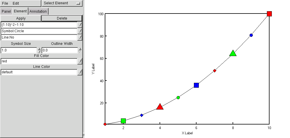
- Although you can still use RGrace for displaying categorical data
there is no support for this in GUI. For example:
ggplot(1:10,(1:10)^2,size=unit(c(1,2),"char"),
gp=gpar(fill=c("red","green","blue")),pch=as.integer(c(21,22,23,24)))
will profuce a picture like this ,
where parameters for the first symbol only is reflected in "Element"
page.
Thanks.
Paul Murrell - for grid package.
Duncan Temple Lang - for RGtk and RGtkGlade packages.
Lyndon Drake Packaging,Martyn Plummer and Duncan Temple Lang - for
gtkDevice package.
And all R-project team for great data analysis software.
Feedback